ASTM E2554 Standard Practice for Estimating and Monitoring the Uncertainty of Test Results of a Test Method in a Single Laboratory Using a Control Sample Program
9. Multiple Readings per Time Period
9.1 Example 1 - Absorbance of Radiochromic Dosimeters:
9.1.1 Over a period of several days, different sets of three dosimeters were irradiated to the same nominal dose. The irradiation was conducted under standard conditions at a single irradiator facility. Possible sources of random errors could include intrinsic variation in dosimeter response and day-to-day variations in the physical environment, for example, temperature, positioning of dosimeters within the irradiator, and shielding. The data was presented in Guide E 1707.
9.2 Table 1 consists of three dosimeters irradiated and measured on a single day. Nine time periods are shown. The averages and standard deviations are computed for each time period.
9.3 Prepare a standard deviation control chart.
NOTE 2 - Ranges could have been computed instead of standard deviations and a range control chart would be prepared.
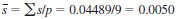
9.3.1 Compute the average of the standard deviations (p test periods):
NOTE 3 - If the standard deviations in many of the samples were zero, then we recommend replacing the values of 0 with a value calculated as: Half-interval √3. In this case the intervals are 0.001 and the half-interval would be 0.0005. Then the estimate of s in place of zero would be 0.0005/1.732 = 0.00028.
9.3.2 The control limits for the standard deviation control chart are found as:
9.3.2.1 The control chart factors B3 and B4 for sample sizes up to n=6 can be found in Table 2. For larger sample sizes see Manual 7.
9.3.3 The control chart is prepared to evaluate the within-sample or time period variation. Control limits as computed are displayed.
9.3.4 The standard deviation chart is examined for unusual values. No readings appear to be unusual.
9.4 A control chart for means is prepared by plotting the means.
9.4.1 The sample means are averaged. The grand average,
 is 0.2878.
9.4.2 The control limits for the means control chart are found as:
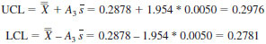
9.4.2.1 The control chart factors A3 for sample sizes up to n=6 can be found in Table 2. For larger sample sizes see Manual 7.
9.4.3 The control chart limits are plotted as presented in Fig. 2.
9.4.3.1 Examination of the means control chart is conducted to determine whether variation between periods appears to be greater than expected from within sample variation. In this example, there are samples just at, and even beyond, the control limits, which is an indicator that the variation over time is much greater than would be expected based only on within-sample repeatability.
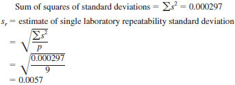
9.5 Estimate the within sample standard deviation. This is an estimate of a single laboratory repeatability standard deviation.
9.5.1 A direct estimate of single laboratory standard deviation is calculated based on the "pooled" variances. This is found by: calculating the squares of each standard deviation; summing the squares; dividing by the number of samples; and taking the square root. In this example:
9.5.2 An alternative estimate of single laboratory repeatability standard deviation can be computed from the average s as:

NOTE 4 - When ranges are used instead of standard deviations, an estimate of sr is found from the average range. In this example, the average range would be found as 0.0097 and the estimate of standard deviation is then found:

where:
 = average range.
9.5.2.1 Factors c4 and d2 for sample sizes up to n=6 can be found in Table 2. For larger sample sizes see Manual 7.
9.6 Between Time or Sample Variation:
9.6.1 Since there is a between sample or between time variation, an estimate of the between time standard deviation is then computed. First the standard deviation among the sample averages is found. This was computed as 0.00590.
9.6.2 The Stime is then computed as:
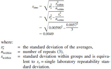
NOTE 5 - If the difference under the radical sign is negative, meaning the estimate of stime(2) is negative, then this may be interpreted as indicating that the variation associated with time is negligible and the estimate of Stime is set to zero.
9.7 The Uncertainty standard deviation is estimated from a single time and a single repeat.

NOTE 6 - This value is equivalent to an estimate of intermediate precision based on multiple time periods.
9.8 An uncertainty control chart is then prepared to monitor future samples. All the initial values should show in control state. The Uncertainty Control Limits are established as defined in Eq 12 and 13 and added to the chart (Fig. 3). First we compute the standard deviation for sample averages assuming there is variation due to time and repeatability. This is an estimate of the uncertainty associated with samples, not individual test results, and is found as:
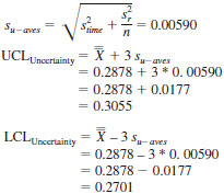
NOTE 7 - The use of the multiplier of 3 is in keeping with traditional control charting practices and are interpreted in a similar manner when used to monitor the process.
NOTE 8 - The initial calculation of the uncertainty standard deviation for samples, Eq 11, is mathematically equivalent to the standard deviation of the averages,
 .
.9.8.1 Averages should continue to be plotted on the uncertainty control chart. If any points go beyond the limits this should be a signal to investigate for possible causes. An unusual number of points at or beyond the limits may indicate that the estimate of uncertainty is too small and should be recalculated.